(figure inspired from Lighthouse3d).
The first OpenGL API appeared in 1992, but the version 3.0, introduced in 2008, started to consider the previous API as deprecated (see ). The legacy API mainly relied on the usage of fixed fonctionnalities: hardware features controled by some predefined parameters. On the other hand, the modern API relies on some programmable stages, the shader programs, which enable the developers to express almost any effect they can imagine. This tutorial is intended to illustrate the modern way of using OpenGL.
However, this modern way can also be applied to some legacy versions, even if this is not mandatory. This tutorial tries not to be dependant on any peculiar version of OpenGL in order to be usable on many platforms, including legacy ones or WebGL. Although this tutorial can mostly work with the legacy API, no assumption is made about any knowledge concerning it. Only the main principles are explained here; the details of each API function can be obtained on the reference pages.
The OpenGL API itself is not specific to any programming language and the examples which are provided here use both C and JavaScript (WebGL). A peculiar attention has been given to make them look very similar; that's why the code itself does not use best C neither JavaScript coding style. Actually, these examples do not focus on the programming language but rather on the common usage of the OpenGL API. The explanations which are given here directly refer to the C source code, but they can be easily understood when dealing with the JavaScript version, since the naming conventions and the comments are similar.
Here is an archive of this OpenGL/WebGL source code and data:
The purpose of this first program is to describe the execution environment prepared for this tutorial.
It relies on the TransProg library () which, amongst many other things, provides an OpenGL Core context and its API (as described in ) and some features to help 3D development.
In order to build the following test programs, the first step consists in generating the makefile by invoking the script
python configure.pyThen the command
python configure.py --makewill actually build the programs. This last command has to be rerun every time a change is made in the source code of a test program.
The limited set of features used in this tutorial is exposed through the
openGlCoreTutorial.hheader file. Each example program includes this file and defines the following functions
  void OpenGlCoreTutorial_init(void);
  void OpenGlCoreTutorial_redraw(void);
  void OpenGlCoreTutorial_keyboard(const char *key);
  void OpenGlCoreTutorial_idle(void);
which are automatically called on purpose. They should use functions prefixed with OGLCT_ (also provided by openGlCoreTutorial.h) to interact with this peculiar execution environment.
Some other utilitarian features are provided by the openGlCoreUtils.h header file. These features are independent from the execution environment and can be easily reused in a different development context.
When running this first program test00_executionEnvironment no OpenGL drawing really occurs, except the changing background colour; we only get text messages in the console to trace the various invocations. The only thing to do here is to read the source code and its comments in order to understand the messages appearing in the console.
The purpose of this program is to introduce the minimal resources needed to produce a simple OpenGL drawing. This is the most important step in understanding the OpenGL pipeline since every next step consists in adding features to the general procedure described here.
The drawing process takes place in our OpenGlCoreTutorial_redraw() function. The actual drawing command
glDrawArrays(GL_POINTS,0,vertexCount);asks for drawing vertexCount vertices as points. The way this drawing is performed is controlled by the command
glUseProgram(program);which specifies the shader-program to use. This shader-program is built from the vertex-shader and fragment-shader source codes provided at the beginning of the file. Each vertex, provided as the v_Vertex input of the vertex-shader, is made of two floating-point values (type is vec2). This pass-through vertex-shader simply assigns this input vertex to the gl_Position built-in output variable (which is made of four floating-point values). This output variable will generate fragments (aka pixels) which colours are controlled by the fragment-shader. Our fragment-shader simply assigns the same colour, the u_Rgb uniform (aka global variable), to the gl_FragColor output variable (which is made of four floating-point values) which determines the colour that will be displayed on the screen. To provide all the parameters required by our shader-program, the command
glUniform3f(u_Rgb,rgb[0],rgb[1],rgb[2]);sets the three floating-point values of our u_Rgb uniform and the command
glBindVertexArray(vao);binds the vao vertex-array which should have previously been prepared in order to associate the input variable v_Vertex with a buffer containing vertexCount vertices (here, pairs of floating-point values). In case this feature is not available, on an old version of OpenGL for example, its effect is emulated by a function call which will be explained later.
The main purpose of our OpenGlCoreTutorial_init() function is to prepare all the resources needed by our OpenGlCoreTutorial_redraw() function. The shader-program is built from the vertex-shader and fragment-shader source codes described above. This build consists in several steps, hidden in the Shader_buildProgram() utilitarian function, but is straightforward and will not be discussed in detail here. The only noticeable thing added by this function over the standard build steps is detecting the current OpenGL version and inserting a preamble into the shader source codes. This preamble mainly consists in defining macros in order to make the source code reasonably portable between legacy and modern shading language versions. After having built the shader-program, we obtain two indices which refers to the u_Rgb uniform and the v_Vertex input variable of this shader-program. As previously stated, the v_Vertex values are extracted from a buffer stored on the graphics card. Thus we prepare pairs of floating-point values (the vertices) in a temporary array; then we create a vertex-buffer-object (vbo) and fill it with our data. These vertices are now stored on the graphics card in a buffer that could be read by a shader-program. In the same manner we create a vertex-array-object (vao). Its main purpose is to associate the input variable v_Vertex with the previously created buffer. Doing so, it is necessary to tell OpenGL that each v_Vertex value is obtained by using two floats from the associated buffer (see our setupVertexArray() function). Everything is now in place for the drawing to take place.
The drawing obtained in this simple example consists in a set of green points regularly spread over the rendering window. Looking at the way the vertices are computed, we see that their coordinates range from -0.9 to 0.9 with a regular step in both the x and y direction. This matches the fact that the rendering viewport is accessed by the gl_Position vertex-shader built-in output variable ranging from -1.0 to 1.0 horizontally (from left to right) and vertically (from bottom to top).
n.b.: vertex-array-objects may not be available on some legacy OpenGL implementations, so we propose a workaround. If this feature is available, the setupVertexArray() function is called only once to initialise the vao; it is then simply bound at every drawing. In case this feature is not available, we simply call the same function at every drawing (the purpose of the vao binding would have been to recall the settings provided here, so we simply repeat them every time they are needed).
Exercise: how could we change the colour of the whole set of points?
Exercise: how could we assign each point its own colour?
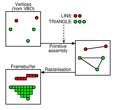
In the previous example, we just saw how to provide OpenGL with all the data necessary to obtain a drawing; but we do not have to specify every single point on the screen. This program introduces the concept of drawing primitive which makes OpenGL generate many fragments (aka pixels) from a few control points provided as vertices.
(figure inspired from
Lighthouse3d).
Our source code is very similar to the previous one except that in our OpenGlCoreTutorial_redraw() function, the drawing command has been changed to
glDrawArrays(drawingPrimitive,0,vertexCount);where drawingPrimitive is assigned with GL_POINTS, GL_LINES or GL_TRIANGLES from our OpenGlCoreTutorial_keyboard() function. Of course, the vertices we provide in the vertex-buffer-object depend on the chosen primitive (see our updateVertexBuffer() utilitarian function).
Exercise: how could we draw vertical lines instead of horizontal ones?
Exercise: how could we draw a checker board instead of only one rectangle made of two big triangles?
Till now, our drawings only took place in a two-dimensional plane; this program introduces the depth-buffer (or Z-buffer) provided by OpenGL in order to deal with the representation of a three-dimensional space on the two-dimensional screen.
Our program now draws several shapes instead of just one. These shapes are simple rectangles (made of two big triangles as in the previous example) but each vertex has three coordinates; x and y have the same meaning as before and z represents a depth value ranging from -1.0 (foreground) to +1.0 (background). This depth value influences the drawing according to the
glEnable(GL_DEPTH_TEST);or
glDisable(GL_DEPTH_TEST);setting used in our OpenGlCoreTutorial_redraw() function. The OpenGL framebuffer, which contains the drawing that will finally appear on the screen, stores for each pixel a depth value which does not appear on the screen but which is tested each time a fragment is about to be drawn. If this incoming fragment has a depth value which is farther than the depth value already present for this pixel in the framebuffer, then the framebuffer is left unmodified. On the contrary, if this incoming fragment has a depth value which is nearer than the depth value already present for this pixel in the framebuffer, then this pixel is overwritten by the colour and depth values of the incoming fragment. Doing so, whatever the drawing order is, only remain visible on the screen the pixels which are not hidden by any nearest object; this offers the ability to represent three-dimensional scenes in a quite natural way. Of course, before every rendering the
glClear(GL_COLOR_BUFFER_BIT|GL_DEPTH_BUFFER_BIT);call resets all the framebuffer to the default colour and the farthest depth.
To enable experimentation, our OpenGlCoreTutorial_keyboard() function can control the enabling of this depth test and can modify the depth value associated with the black rectangle. The informations representing the various rectangles drawn here are stored in some ExampleShape data structures but are very similar to what was used in the previous examples. When specifying the content of a rectangle vertex-buffer-object (see our updateVertexBuffer() function), and especially each time the black one receives a new depth value, we adjust its width and height so that farthest ones remain partially visible while partially hidden by nearest ones.
The only thing to do here is to understand that the black rectangle, which is always drawn first, is not overwritten by any other rectangle, although it is drawn after, until its own depth is less than the depth of this other one.
In the previous example, each time a shape had to be moved on the screen we regenerated the content of its vertex-buffer-object. It is however possible, and even recommended, to describe the geometry of each shape once for all and to use the vertex-shader to transform the vertices during the rendering.

(figure inspired from
Lighthouse3d).
Exercise: how could we reduce the number of trigonometric operations needed to rotate the shapes?
Although our previous example used three-dimensional coordinates, the drawing was only made of two-dimensional shapes stacked along the third dimension. To deal with real three-dimensional shapes placed and moving freely in a three dimensional space, homogeneous coordinate matrices are very commonly used. Moreover OpenGL hardware and shader programs have built-in instructions to perform efficient computations with such matrices.
Some detailed explanations about homogeneous coordinates can be found
here:
Because we work in a three-dimensional space, we need four-dimensional square matrices (made of sixteen floating-point numbers). They can be composed so that one single resulting matrix contains the accumulation of many transformations such as translation, rotation, scaling, projection... The main purpose of such a matrix is to transform a three-dimensional point or vector. The functions for all of these common operations are prefixed with Matrix4_ in the openGlCoreUtils.h file.
In our program, each ExampleShape structure is now dotted with such a matrix which is initialised in our OpenGlCoreTutorial_init() function and which changes in our OpenGlCoreTutorial_idle() function. Of course, this matrix is sent to the u_LocationMatrix uniform variable of our shader-program every time a shape is rendered in our OpenGlCoreTutorial_redraw() function. As we can see in our vertex-shader source code, this matrix is simply used to multiply each vertex of the rendered shape (a cube stored once for all in its vertex-buffer-object).
Exercise: how could we translate the black shape using the keyboard?
So far, all the three-dimensional coordinates took place in a volume ranging from -1.0 (left, bottom or foreground) to +1.0 (right, top or background). Actually, OpenGL produces rendering fragments from the gl_Position vertex-shader built-in variable which is expressed in the so-called Normalised Device Coordinate system (NDC). If we want our shapes to be placed anywhere in a wider space, we need a projection matrix to transform these coordinates to the NDC system. Moreover, to correctly perceive the relative distances in a rendered scene, the farthest shapes should appear smaller than the nearest ones, then this matrix must describe a perspective projection.
The u_ProjectionMatrix uniform variable of our vertex-shader source code now transforms the vertices of the shapes previously located in space with the u_LocationMatrix uniform variable. This projection matrix is computed, once for all these shapes, at the beginning of our OpenGlCoreTutorial_redraw() function, but is used by all of them. When computing a projection matrix, the Matrix4_perspectiveProjection() utilitarian function (see openGlCoreUtils.c) requires:
Some detailed explanations about transformation and perspective matrices can
be found here:
(code mainly relates to legacy OpenGL but explanations are still valid).
To enable experimentation, our OpenGlCoreTutorial_keyboard() function can control the switch between a NDC (identity) or perspective projection matrix. The only thing to do here is to observe and understand the effect of using these two different projection matrices to render the same scene.
Even if the previous perspective projection matrix offers a natural view for shapes freely located in any three-dimensional space, it implies that the whole scene has to be placed in the visible volume defined by this perspective. To simulate a navigation through this scene it should be necessary to move all the shapes so that they appear under different angles and positions in this visible volume. It is much more convenient to define a view-point which can move in the three-dimensional space as shapes do, and to take it into consideration while transforming the vertices. Of course, the location of this view-point is defined by another homogeneous coordinate matrix.
At this stage we must pay a peculiar attention to the different coordinate systems we use. Except NDC which is imposed by OpenGL as output for the vertex-shader (gl_Position built-in variable), any other coordinate system could be used to represent anything (shape location, view-point...) as it is just a matter of matrix multiplication. As a reminder, NDC uses this convention:
In this example source code, our viewPoint variable is a four-dimensional homogeneous-coordinate matrix similar to the location variable of our shapes. It is then initialised (in our OpenGlCoreTutorial_init() function) and changed (in our OpenGlCoreTutorial_keyboard() function) in a very similar way as for the shapes. To ease interaction, the OGLCT_controlViewPoint() function also gives our execution environment the ability to change this view-point matrix according to mouse movements. As already said at the beginning of this part, the purpose of this view-point matrix is to simulate the fact that the whole three-dimensional scene moves around the OpenGL rendering point from which the perspective projection is computed. Thus, the vertices of the shapes must not only be transformed by the location matrix but also by the inverse of viewPoint matrix. Moreover, because the perspective projection matrix use different conventions for its axes, this transformation must include this switch. Our OpenGlCoreTutorial_redraw() function then uses the Matrix4_computeView() utilitarian function to obtain the so-called view matrix representing the inverse of the view-point and the axis switch. Multiplying this view matrix by the location of a shape gives the so-called modelView matrix which is finally sent to our shader-program as our u_ModelViewMatrix vertex-shader uniform variable. One can notice that, except the name of this uniform variable, nothing changes between this vertex-shader source code and the one in the preceding example; the values stored in the matrices have a different meaning but the computations performed by the shader-program remain the same.
Some detailed explanations about transformation matrices can
be found here:
(code mainly relates to legacy OpenGL but explanations are still valid).
The only thing to do here is to observe and understand the effect of the keyboard and mouse interactions on the view-point.
Although you should have noticed in the previous example that the ability to move the view-point in the scene helps perceiving the relative size and position of the shapes, one can hardly see the geometric details of a shape. As every fragment of a shape has the exact same colour, only the outline of this shape gives informations on its geometry. The purpose of this new program is to provide every fragment its own colour in order to highlight geometric details.
A really important feature of OpenGL, that we have not really used for now, stands in the fact that, even if we only provide data to the vertex-shader (via vertex-buffer-objects), an interpolation of these values is automatically generated over the constitutive fragments of an OpenGL primitive. Position in camera space is an obvious (and the main) effect of this interpolation but it could be done with any data; colours will be used here.

(figure inspired from
Lighthouse3d).
Our fragment-shader source code no longer uses a uniform variable to assign the fragment colour but instead relies on our f_Colour input variable. This one comes from the f_Colour ouput variable of our vertex-shader source code. Because a few vertices involved in an OpenGL primitive (three for a triangle here) produce many fragments, the value of f_Colour obtained in the fragment-shader is not exactly one of these given to a vertex but an interpolation between these three values. The values of the v_Colour input variable used in our vertex-shader source code come from a supplemental colourVbo vertex-buffer-object. This one is similar to the one containing the vertices, vertexVbo, and is also associated with the vertex-array-object of the shape (see our OpenGlCoreTutorial_init() function).
Now that a shape uses many different colours, it becomes easier to perceive its geometry.
Exercise: how could we assign a different colour to each face of a cube instead of a different colour for each vertex?
Even if the varying colours of the previous example help us perceiving the geometry of the shapes, one must admit that their multicolour aspect is far from natural. Now that we know about interpolation of fragment-shader input values from their vertex-shader output counterparts, we can use this feature to compute the effect of a light source on a surface. This is called "shading" and it represents the original purpose of shader-programs.
There exist many ways to simulate lighting effects; we use here a simple set of very common features (Blinn-Phong shading):

Because this lighting model relies on a surface normal, each vertex has its own normal vector (v_Normal vertex-shader input variable) which is provided by a vertex-buffer-object as the geometry is. Our vertex-shader source code now produces two output variables, f_Normal and f_CamPos, which are interpolated and used as input variables in our fragment-shader source code. They represent the normal vector and the position of the fragment expressed in the camera coordinate system. The u_HeadLight uniform contains the light position in the same coordinate system so we can perform all the lighting computations described above with these local variables:
When describing the geometry of a shape, in our OpenGlCoreTutorial_init() function, we have to fill its normalVbo vertex-buffer-object which is associated with the vertex-array-object of that shape. One can notice that some vertices have identical positions but different normal vectors because they take place on different faces of the shape.
Our OpenGlCoreTutorial_keyboard() function can control the location of the light source relative to the view-point (thus expressed in the camera coordinate system). Moving this head-light as well as moving the view-point illustrate our lighting model by producing different shades of the same colour depending on normal, view and light vectors (disabling the animation can help the observation). This makes the shapes look quite natural and easy to perceive.
Exercise: how could we simulate a coloured light instead of a pure white one?
Exercise: how could we take into account a second light with a fixed position in the scene?
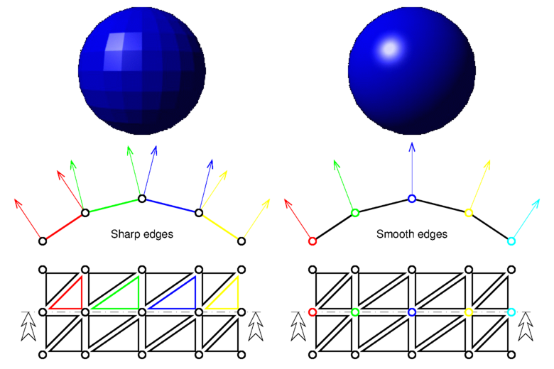
When describing a surface made of adjacent triangles (a triangle mesh), many vertices have the same position but take place in different triangles. To make these triangles form a sharp edge, the superposed vertices must have different normal vectors to produce distinctive lighting effects; this was the case for the different faces of the cubes in the previous example. On the other hand, if these triangles are small parts of a smooth surface, the lighting effect must vary continuously on this whole surface; it means that the superposed vertices must have exactly identical properties, including their normal vector, and this was the case for the two triangles forming the same face of a cube in the previous example. In this latter case, describing the whole surface leads to transmitting a lot of redundant informations to OpenGL, which implies a lot of redundant computations too. It is therefore recommended to describe all the vertex data once for all and to form triangles by referring to these vertices via their integer index into their vertex-buffer-object. For example, one can describe a first triangle composed of the first, second and third vertices, and a second triangle composed of the second, third and fourth vertices; these two triangles share two vertices so their common edge will look smooth. If we want some of the edges in the mesh to look sharp, then we simply duplicate their superposed vertices to give them different normals; each triangle refers to the vertex indices corresponding to the ones with the appropriate normals.
This program uses exactly the same shader-program than the previous example. The only difference stands in the way the vertex-array-object are composed. They now refer to a supplemental vertex-buffer-object containing the indices of the vertices forming the triangles. In our OpenGlCoreTutorial_init() function, a sinusoidal surface is generated by computing the position and normal of each vertex. The mesh is formed as a grid by composing triangles in the x,y plane while z is the elevation. Some other shapes can be obtained from external tools that constitute and generate such meshes; the utilitarian function Mesh_load() makes some of them available. Our OpenGlCoreTutorial_redraw() function now uses the command
glDrawElements(GL_TRIANGLES,indexCount,GL_UNSIGNED_INT,NULL);to draw such a mesh. It uses indexCount integer indices, taken from the appropriate vertex-buffer-object of the currently bound vertex-array-object, to enumerate the vertex data forming the triangles.
One can notice that smooth surfaces, especially when they are generated from apropriate tools or data, appear with a quite realistic aspect. This effect is reinforced when moving the head-light thanks to the OpenGlCoreTutorial_keyboard() function. It is also noticeable that, depending on the view-point and as soon as the normals are correctly generated, there is no need to provide a huge amount of vertices to make the shape look smooth. This can be observed by comparing the three generated sinusoidal surfaces.
Exercise: since by default only counterclockwise oriented triangles are rendered (this can be changed on some versions of OpenGL), how could we make our sinusoidal surfaces visible from below instead of above?
Now that we are able to represent shapes in a way that makes them easily recognisable, we can introduce graphical effects to bring, for example, a peculiar atmosphere into the scene. Because the shader programs enable us to compute almost anything, provided that we know the appropriate equations and parameters, this feature can be used to alter the colours in order to produce the desired visual effect. This example simply simulates the effect of two different fog effects:
Our fragment-shader source code begins with the usual computation of the lighting effect but this colour is not directly applied to the fragment. A fog intensity is then computed and the resulting colour of the fragment is a mix varying continuously from the lighting colour (fog intensity is 0.0) to the fog colour (fog intensity is 1.0). This fog intensity is generally a function of the distance along which the fog is traversed by the view vector. For a global fog this is simply the distance to the fragment, but when it comes to a volumetric fog we have to determine the length of the intersection between the view-direction and the the fog volume. Actually, when switching to the volumetric fog with the OpenGlCoreTutorial_keyboard() function, one can notice that the effect of the fog is less visible at the edge of the sphere than in its middle.
To achieve a convincing effect, the background should have the same colour as the fog; in this program, this is the case only for the global fog. Actually, the details which are supposed to be far away seem to be fully faded by the fog.
Exercise: how could we make the volumetric fog visible where there is no shape?
The effects we use to determine the colours of the shapes do not need to be look realistic. A famous one is the so-called toon-shading effect which tends to make the shape appear as if they were drawn in a comic strip with very few colour shades.
As visible in our fragment-shader source code, this effect simply computes the diffuse intensity as usual but transforms it to obtain several discrete colour levels. These ones produce large homogeneous colours which exaggerate the effect of the light direction on the normals.
A central feature of OpenGL stands in the ability to apply textures. This means that a picture can be mapped on a shape, as we put up some wallpaper on a wall, to give it many coloured details. A picture taken from a real object and correctly mapped on a simplified geometry can be sufficient to make this shape look natural and easily recognisable. Moreover it is more efficient than describing this shape as many geometric details associated with their own colour.
A texture-object is an OpenGL resource representing a picture (some variants exist). It is generally loaded once for all into the OpenGL device:
  glGenTextures(1,&texture);
  glBindTexture(GL_TEXTURE_2D,texture);
  glTexImage2D(GL_TEXTURE_2D,0,GL_RGB,texWidth,texHeight,
               0,GL_RGB,GL_UNSIGNED_BYTE,texData);
  ...
(see our OpenGlCoreTutorial_init() function).glUniform1i(u_TexUnit,0); // GL_TEXTURE0 glActiveTexture(GL_TEXTURE0); glBindTexture(GL_TEXTURE_2D,texture);(see our OpenGlCoreTutorial_redraw() function).

(figure taken from
blog.tartiflop).
The square which is generated in this example has very simple texture coordinates corresponding to the corners of the texture. When a complex geometry is loaded from a file produced by a dedicated tool, the texture coordinates are generally exported by this tool, as normal vectors are.
Exercise: apply a transformation to the texture coordinates in our fragment-shader source code and observe how the mapping is modified.
As mentioned in the preceding example, an OpenGL device has several texture units. This means that several textures can be bound and used at the same time when rendering a shape. The colours picked from each of them can then be combined to produce the rendering colour of the considered fragment.
The changes needed in the shader-program source codes are quite straightforward. An additional uniform variable indicates another texture unit and a new vertex-buffer-object provides some other texture coordinates as vertex-shader input variable. Actually, a vertex can have distinct texture coordinates for the different textures the shape refers to.
Our example uses as second texture a series of pictures producing an animation. All of these are loaded once for all in our OpenGlCoreTutorial_init() function and the switching between them, occurring as time goes by in our OpenGlCoreTutorial_redraw() function, only relies on the binding operation to the appropriate texture unit. Because the set of pictures used in this example is only made of a single grey channel, the created textures only contain information for their red channel (no green, neither blue). Consequently, our fragment-shader source code duplicates this red channel towards the green and blue ones, so that we can easily modulate the rendering colour with this shade of grey.
Exercise: in this specific example, couldn't we get rid of the vertex-buffer-object providing the texture coordinates for the second texture unit?
One may have noticed that, starting from the beginning of this tutorial, all the colour informations assigned to the fragments are made of four components. Three of them are the usual red, green and blue channels and we systematically add the value 1.0 as fourth channel. This so-called alpha-channel is generally used in order to simulate transparency. It ranges from 0.0, meaning that the fragment should be totally transparent, to 1.0, meaning that it should be totally opaque.
A first and simple usage of this alpha-channel stands in an all-or-nothing test of its value against a threshold to decide if the fragment will be written to the framebuffer or discarded. Our fragment-shader source code uses the discard keyword to do so, based on the alpha-channel taken from a texture. Actually, when generating, with the appropriate tool, a rectangular picture dedicated to become a texture, one can provide this all-or-nothing information in a supplemental alpha-channel in order to specify the only pixels that constitute the actual drawing. It is the case, in this example, for the leaf and wire-fence textures.
Another common usage of this alpha-channel is more subtle and uses the intermediate values (between 0.0 and 1.0) to make some shapes visible but shaded through some others that are semitransparent. This technique is called alpha-blending and is performed, when enabled, by the OpenGL device when a fragment is written into the framebuffer. The colour of the incoming fragment does not replace anymore the preceding one (when the depth test succeeds) but is instead combined with it to produce the new colour to be stored in the framebuffer. The very commonly used call
glBlendFunc(GL_SRC_ALPHA,GL_ONE_MINUS_SRC_ALPHA);which is made in our OpenGlCoreTutorial_init() function tells that this combination is computed like this:
stored_colour = incoming_colour * incoming_alpha + previously_stored_colour * ( 1.0 - incoming_alpha )This equation is coherent with the fact that an incoming fragment is totally transparent when its alpha value is 0.0 an totally opaque when it is 1.0. However, this technique has a drawback: the rendering of the shapes is not anymore order independent (it was, till now, thanks to the depth-buffer). Drawing a shape which is behind another semitransparent one will not produce the same resulting colour if it is rendered before or after this one. To overcome this artifact it is necessary to take the semitransparent shapes apart from the opaque ones. First, the opaque shapes are rendered as usual, then the blending effect is enabled and the semitransparent ones are rendered from the farthest to the nearest. This sorting is necessary to make the colours of the nearest shapes more visible than those of the farthest ones. But, as visible in our OpenGlCoreTutorial_redraw() function, this sorting relies only on the position of these shapes; and, as their geometries can be intricate, some of their respective fragments might not be correctly sorted. If this occurs, the depth test could discard some fragments that should have appeared behind (thus before) some nearest semitransparent others. For this reason, our OpenGlCoreTutorial_redraw() function disables the writing to the depth-buffer when it enables the blending effect. Doing so, the depth test only occurs against the previously rendered opaque shapes, and the semitransparent fragments that are not hiden by the opaque shapes are always rendered even if they are not correctly sorted.
Our OpenGlCoreTutorial_keyboard() function can be used to enable or disable the sorting of the semitransparent shapes in order to show the alpha-blending artifact. Moving the view-point highlights the fact that this sorting has to be done at every rendering; some shapes that are correctly rendered under a certain view-point could produce incorrect colours under another view-point.
As a geometry is described by a triangle mesh, many small triangles are necessary to represent very thin details. This huge amount of data to access and process during rendering is a very common performance bottleneck. An alternative exists to make some geometric details perceivable without increasing the triangle count; this relies on a texture which contains normal coordinates instead of colours. It provides each fragment with its own normal, based on a texture lookup and not anymore as an interpolation of vertex normals. Since normals are central to lighting, a single triangle, on which an appropriate normalmap texture is mapped, contains many shading effects which are sensible to light and view-point. This reasonably simulates what could be perceived if there were many more geometric details.
In our program, the pink and blue calves are usual triangle meshes. One can see that, since it is a decimated version, the blue one contains much less triangles than the pink one. In particular, the details of the neck and the head totally disappear. When generating the decimated version from the detailed one, a normalmap texture has also been computed from the detailed vertex normals. It is similar to a usual texture except that the three components do not describe a colour but a normal vector. The green calf in our program uses this normalmap texture and, although it is described by the same decimated geometry as the blue one, it shows many shading details on its neck and on its head. In the same manner, the ground is a perfectly flat square associated with a normalmap texture describing variations around the vertical (z) main normal.
Our normalmap specific vertex-shader does not handle normal coordinates anymore but instead uses texture coordinates for the normalmap texture. Our normalmap specific fragment-shader performs a lookup in this texture and rescales the three components from the range [0.0;1.0] (suitable for colours) to the range [-1.0;1.0] (suitable for normals). Then this normal vector is transformed by the model-view matrix as it is usually done at the vertex-shader stage. Starting from here the usual lighting computation can be performed.
Moving this head-light as well as moving the view-point illustrate that using these normalmap textures is quite different from using traditional textures (which can be used conjointly). Two fragments of the same triangle can appear respectively dark and light under a certain light position and view-point, and with the opposite shades under other circumstances.
Exercise: reuse the normalmap texture as a colour texture and try to understand the colours which are displayed on the shapes.
The preceding program used normalmap textures that were specific to their associated geometries, so they naturally contained normals which were expressed in the same vector basis as their geometry. This is quite reasonable for the calf normalmap texture because it makes no sense to reuse it with another geometry. But concerning the brick pattern of the ground, one could decide to reuse it on a different support (a wall, a cylinder, a complex shape...). In this case, the chosen vertical main axis (z) around which the normalmap texture describes variations does not match anymore the surface of the shape. This normalmap texture should be considered as expressed in a three-dimensional vector basis defined by:

As seen in our fragment-shader source code, the normal vector in this basis is just taken as the interpolation of the vertex normals. The tangent vector is chosen, in our tangentBasis() fragment-shader function, along the texture coordinate variations and the cotangent vector is deduced to form a right-hand basis. The normal perturbation picked from the normalmap texture is then transformed in this coordinate system to provide the actual normal vector for the considered fragment. One can notice that, since the shape can be complex, the tangent basis is not the same for every fragment.
Enabling and disabling the normalmap texture mapping with our OpenGlCoreTutorial_keyboard() function helps perceiving the improvement of this rendering technique over the usual texture mapping. Of course such textures have to be generated from an appropriate tool but, as shown here, they can be reused in various contexts.
Exercise: reuse the normalmap texture as a colour texture and try to understand the colours which are displayed on the shapes.
Till now, every drawing took place in a framebuffer associated with a window, but OpenGL enables us to create other framebuffers that may not be directly displayed on the screen. A common usage consists in reusing this offscreen framebuffer as a texture which is mapped on a geometry for the final rendering into a window. This dynamic texture can be used to simulate visual effects; a mirror for example.
In this program, when it comes to the shape using this dynamic texture, our OpenGlCoreTutorial_init() simply creates an OpenGL texture-object as usual except that no data is provided; it is just created with the required size and a black content. Then we create an OpenGL framebuffer-object with its own depth-buffer and the preceding texture as colour-buffer. When our OpenGlCoreTutorial_redraw() needs to update this texture, we simply bind this specific framebuffer with the call:
glBindFramebuffer(GL_FRAMEBUFFER,fbo);and generate the desired drawing as usual. Binding no specific framebuffer with the call:
glBindFramebuffer(GL_FRAMEBUFFER,0);produces the following rendering in the window back again.
Because in this example we simulate a mirror effect, the mirror content is the drawing of the same scene under a different view-point. Our OpenGlCoreTutorial_redraw() computes this new view-point using a symmetry through the mirror plane. Then the projection matrix for this peculiar rendering takes into account the size of the mirror and the off-axis offset: we take place behind the mirror look at the scene through it as if it was a window. The resulting offscreen rendering takes place in the associated texture so that it is mapped as usual onto the mirror geometry during the final rendering.
Till now, the mirror effect put aside, textures were considered as internal properties of the shapes and were not dependent on the environment. However, there exists a peculiar kind of texture-object, the so-called cube-texture, which is actually made of six square pictures considered as a whole. They are commonly used to represent the environment as projected onto the internal surface of a surrounding cube.
A first and simple usage of such a cube-texture is the rendering of a skybox. The idea is to entirely fill the background with a texture in order to represent the details which are considered to stand at an infinite distance from the view-point. The skybox shape is a simple cube without any normal nor texture coordinate. To keep this cube always centred around the view-point, our skybox vertex-shader source code uses a trick: while transforming the vertices with the view-matrix, they are considered as vectors (the fourth homogeneous coordinate is set to 0.0) so that the view-matrix does not induce any translation but only a rotation. As visible in our drawSkybox() function, the rendering of this shape will not alter the depth-buffer, thus any next shape to be rendered will be considered in front of it; that is why the actual size of this cube does not matter. When it comes to the skybox fragment-shader source code, we simply use the view vector (from the centre of the cube to a point on its surface) as the cube-texture coordinate, nothing more. Actually, this is a built-in feature for OpenGL to select the appropriate pixel of the appropriate face of the cube-texture based on this vector.
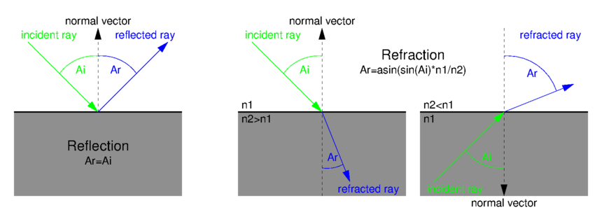
The same idea can be reused to simulate reflection or refraction effects. As shown on the bellow figure, an incident ray on a shape produces a reflected or refracted ray which is re-emanated towards the environment. The colour to be displayed at the incidence point on a reflective or refractive shape depends on this re-emanated vector and is then taken from a cube-texture representing the surrounding environment of this shape (generally the same as the skybox). Our vertex-shader source code simply computes the incident and normal vectors (expressed in the world coordinate system) which are interpolated and reused in our fragment-shader source code. Our u_RefractiveRatio uniform variable controls the desired effect:
If every shape in the scene uses the same cube-texture as the skybox, their reflection or refraction effect can only take the background into account. To make other shapes appear on a reflective or refractive shape, this latter should have its own cube-texture which is updated with its own surrounding environment. Thus, in our OpenGlCoreTutorial_init() function, each of these shapes is provided with a cube-texture and an OpenGL framebuffer-object associated with it. As visible in our OpenGlCoreTutorial_redraw() function, updating such a cube-texture simply consists in generating an offscreen rendering for each of the six faces of the cube. The view-point is chosen as the centre of the considered shape and is oriented according to the considered face. The field-of-view and the width-height ratio of the perspective projection matrix are chosen to make each face coincide with its neighbours.
Switching between the per-shape or the common cube-texture is enabled by our OpenGlCoreTutorial_keyboard() function, as well as changing the refractive ratio.
Exercise: assign the fragment a colour representation of the cube-texture coordinate instead of the actual texture and try to understand the colours which are displayed on the skybox and the shapes.
Exercise: try to detect the total internal reflection effect.
Vertex-morphing simply consists in interpolating a geometry between key-frames. A key-frame describes a deformable shape in a specific pose. The interpolation makes the shape smoothly change from one pose to another as time goes by.
All of the key-frames for a particular shape are very similar: they have to describe the same mesh, only vertex positions and normals vary from one key-frame to another. As seen in our vertex-shader source code, the actual vertex and normal coordinates are the result of a weighted sum of the values for the previous and a next pose (controled by our u_NextPrevRatio uniform variable). Thus, our OpenGlCoreTutorial_redraw() function is responsible for binding the desired previous and next vertex-buffer-objects and for computing the ratio to mix them. One can notice that there is no need to compute these coordinates in the main program and send them to the graphics card; everything is computed in-place by OpenGL.
All the poses are loaded once for all in our OpenGlCoreTutorial_init() function and arranged in order to form an animation cycle. During the rendering, they are used at the same time by several shapes which appear simultaneously in different poses because each one uses its own interpolation parameters.
Exercise: make the fingers move twice before opening the hand.
Drawing many similar shapes in the same scene is generally a performance bottleneck for rendering. Actually it implies a long rendering sequence if which, for each shape, some shape specific parameters are set (via uniform variables) before each triggering of the actual drawing. This leads to more time being spent into the numerous OpenGL invocations than in the actual drawing. When these shapes can be represented as simple spheres, forming a particle system for example, we can use a trick that consists in rendering the whole set of particles as a single shape made of many points; a specific shader-program makes these points appear as lit spheres. A second advantage of this trick is that there is no need to provide a triangle-mesh for these spheres: a single point is changed into an infinitely smooth sphere, whatever its size is on the screen.
Our vertex-shader source code just transmits input vertices to the next shader stage which is in this case the geometry-shader. The main purpose of this new kind of shader is to generate additional vertices from the incoming ones; here, each point is changed into a square made of two adjacent triangles, thus four vertices. These new vertices are computed so that the generated square is facing the camera. Our f_Offset output variable is interpolated and reused in our fragment-shader source code to locate the relative position of each fragment inside this square. Our f_CamPos output variable is identical for the four vertices and represents the centre of this square. Our fragment-shader source code uses our f_Offset input variable to determine if the considered fragment lies within the inscribed disk of the square; if not, the discard keyword prevents the fragment from being drawn. Then we suppose that this disk represents the projection of sphere located at the same place. Thus, the considered fragment should be seen as if it was on the surface of this sphere (not on the square) and some simple geometrical operations give its position and normal. Usual lighting equations can then be used starting from here. A last optional operation consist in adjusting the gl_FragDepth built-in output variable to make the bump of the sphere appear in the depth-buffer. Without this depth adjustment, the sphere is still considered as a flat disk and will let appear some very close shapes that would have been hidden by the surface of the sphere.
Some legacy OpenGL implementations and WebGL do not provide the geometry-shader feature requested here. Fortunately, there exists a workaround. The GL_POINT_SPRITE legacy feature, which is implicitly enabled in WebGL, consists in specifying the gl_PointSize built-in variable from the vertex-shader source code. Doing so, a point is drawn as a square of the specified size in pixels (which must take into account the width of the screen and the projection matrix). On the fragment-shader side, the gl_PointCoord built-in variable provides some kind of texture coordinates for the generated square, from which we can simply deduce an offset relative to the centre of the square. Some of these OpenGL implementations do not either provide the ability to adjust gl_FragDepth.
Exercise: simply draw a black square with its inscribed unicolour disk instead of a sphere.
Exercise: how could we assign each particle its own colour?
Even if lighting equations make the appearance of a shape change according to light and view directions, the resulting colour does not take in consideration the surrounding shapes. A way to make a scene look more natural is to make the shapes cast shadows on each other. This relies on a two-pass rendering. The purpose of the first one is to determine the fragments of the shapes which are directly lit by the light and those which are not; no actual colour rendering is performed, only the depth-buffer is altered. The second pass reuses the previous depth-buffer as a texture providing informations which help determine if a fragment should be fully lit or darken.
The main idea for the first pass is to consider the light source as a camera. Indeed, a light source casts rays on some surfaces that directly face it, as well as a camera receives colours from some surfaces that directly face it. In both cases, only are lit or visible the surfaces which are not hidden by any other ones. So as shown on the below figure, we produce an offscreen rendering of the scene as if it was seen from the light point of view. To keep this example simple, we consider a directional light so that the associated projection matrix is orthographic. This matrix describes a volume that encompasses the whole scene. The resulting depth-buffer is called a shadowmap.

When rendering the second pass, which actually produces the final colours, we also provide the projection matrix used in the first pass (u_ShadowMatrix). Thus, as we transform the vertices in the usual way, we also transform them with u_ShadowMatrix, which produces the fragments that were submitted to the depth-buffer in the first pass. Since we also provide in u_ShadowTexUnit the shadowmap obtained in the first pass, we can compare the depth of such a fragment against the one which is stored in the shadowmap; when the latter is smaller than the former it means that there is an obstacle between the fragment and the light so the considered fragment stands in the shadow. Once this information is known we can alter consequently the diffuse and specular contributions of the lighting equation.
In order to obtain a decent result, some tweaks must be used. First of all, when comparing a fragment against the shadowmap a threshold has to be considered in order to avoid self-shadowing fragments. This is due to the fact that the depth resolution of the depth-buffer is limited, so the stored value is rounded. Moreover, because the shadowmap has also a limited resolution for its width and height, several fragments near to each other in the second pass will refer to the same value in the shadowmap; this leads to a sharp and pixellated shadow border. To reduce the sharp border effect, instead of testing just one pixel in the shadowmap, we use a small patch to average the result of the test on the surrounding pixels. To reduce the pixellated effect, a special texture sampler (sampler2DShadow, which may not be available on some legacy OpenGL implementations) can perform the depth comparison by itself and interpolate the result between the adjacent pixels in the shadow map (has in classical texture lookups).
Exercise: cancel the depth-threshold in order to observe the self-shadowing artifacts.
Exercise: cancel the 5x5 patch in order to observe the sharp edges.